Abstract: This article mainly shares how to build and train convolutional neural networks from scratch using Tensorflow. This way you can use this knowledge as a building block to create interesting deep learning applications.
0. Introduction In the past, I wrote mainly "traditional" machine learning articles, such as naive Bayesian classification, logistic regression, and Perceptron algorithms. In the past year, I have been studying deep learning techniques, so I want to share with you how to use Tensorflow to build and train convolutional neural networks from scratch. In this way, we can use this knowledge as a building block to create interesting deep learning applications in the future.
To do this, you need to install Tensorflow (see the installation instructions), and you should have a basic understanding of the theory behind Python programming and convolutional neural networks. After installing Tensorflow, you can run a smaller neural network without relying on the GPU, but for deeper neural networks, you need to use the computing power of the GPU.

There are many websites and courses on the Internet that explain the workings of convolutional neural networks, some of which are still very good, well illustrated and easy to understand []. I won't explain the same thing here, so before you start reading, please understand in advance how convolutional neural networks work. E.g:
What is a convolutional layer, and what is the filter for the convolutional layer?
What is the activation layer (ReLu layer (the most widely used), S-type activation or tanh)?
What is the pool level (maximum pool / average pool), what is dropout?
What is the working principle of random gradient descent?
The content of this article is as follows
Tensorflow Foundation
1.1 Constants and variables
1.2 Diagrams and Sessions in Tensorflow
1.3 placeholders and feed_dicts
Neural network in Tensorflow
2.1 Introduction
2.2 Data loading
2.3 Create a simple layer of neural network
2.4 Multiple aspects of Tensorflow
2.5 Creating a LeNet5 Convolutional Neural Network
2.6 Parameters that affect the output size of the layer
2.7 Adjusting the LeNet5 Architecture
2.8 Learning Rate and Optimizer Impact
Deep neural network in Tensorflow
3.1 AlexNet
3.2 VGG Net-16
3.3 AlexNet performance
Conclusion
1. Tensorflow basicsHere, I will give a brief introduction to people who have never used Tensorflow before. If you want to start building a neural network right away, or are already familiar with Tensorflow, you can jump straight to Section 2. If you want to learn more about Tensorflow, you can also check out this code base or read the Handout 1 and Handout 2 of the Stanford University CS20SI course.
1.1 Constants and variables
The most basic units in Tensorflow are constants, variables, and placeholders.
The difference between tf.constant() and tf.Variable() is clear; a constant has a constant value, and once it is set, its value cannot be changed. The value of the variable can be changed after the setting is completed, but the data type and shape of the variable cannot be changed.
#We can create constants and variables of different types.
#However, the different types do not mix well together.
a = tf.constant(2, tf.int16)
b = tf.constant(4, tf.float32)
c = tf.constant(8, tf.float32)
d = tf.Variable(2, tf.int16)
e = tf.Variable(4, tf.float32)
f = tf.Variable(8, tf.float32)
#we can perform computaTIons on variable of the same type: e + f
#but the following can not be done: d + e
#everything in Tensorflow is a tensor, these can have different dimensions:
#0D, 1D, 2D, 3D, 4D, or nD-tensors
g = tf.constant(np.zeros(shape=(2,2), dtype=np.float32)) #does work
h = tf.zeros([11], tf.int16)
i = tf.ones([2,2], tf.float32)
j = tf.zeros([1000,4,3], tf.float64)
k = tf.Variable(tf.zeros([2,2], tf.float32))
l = tf.Variable(tf.zeros([5,6,5], tf.float32))
In addition to tf.zeros() and tf.ones() being able to create a tensor with an initial value of 0 or 1 (see here), there is also a tf.random_normal() function that creates a random value containing multiple values. The tensor, these random values ​​are randomly extracted from the normal distribution (the default distribution is 0.0 and the standard deviation is 1.0).
There is also a tf.truncated_normal() function that creates a tensor containing values ​​randomly extracted from the truncated normal distribution, where the lower upper limit is twice the standard deviation.
With this knowledge, we can create weighting matrices and deviation vectors for neural networks.
Weights = tf.Variable(tf.truncated_normal([256 * 256, 10]))
Biases = tf.Variable(tf.zeros([10]))
Print(weights.get_shape().as_list())
Print(biases.get_shape().as_list())
>>>[65536, 10]
>>>[10]
1.2 Graphs and Sessions in Tensorflow In Tensorflow, all the different variables and operations on these variables are stored in the Graph. After you have built a diagram that contains all the calculation steps for the model, you can run the diagram in a session. Sessions can allocate all calculations across CPU and GPU.
Graph = tf.Graph()
With graph.as_default():
a = tf.Variable(8, tf.float32)
b = tf.Variable(tf.zeros([2,2], tf.float32))
With tf.Session(graph=graph) as session:
Tf.global_variables_iniTIalizer().run()
Print(f)
Print(session.run(f))
Print(session.run(k))
>>>
>>> 8
>>> [[ 0. 0.]
>>> [ 0. 0.]]
1.3 placeholders and feed_dicts
We have seen various forms for creating constants and variables. There are also placeholders in Tensorflow that do not require an initial value and are only used to allocate the necessary memory space. In a session, these placeholders can be populated with (external) data via feed_dict.
The following is an example of the use of placeholders.
List_of_points1_ = [[1,2], [3,4], [5,6], [7,8]]
List_of_points2_ = [[15,16], [13,14], [11,12], [9,10]]
List_of_points1 = np.array([np.array(elem).reshape(1,2) for elem in list_of_points1_])
List_of_points2 = np.array([np.array(elem).reshape(1,2) for elem in list_of_points2_])
Graph = tf.Graph()
With graph.as_default():
#we should use a tf.placeholder() to create a variable whose value you will fill in later (during session.run()).
#this can be done by 'feeding' the data into the placeholder.
#below we see an example of a method which uses two placeholder arrays of size [2,1] to calculate the eucledian distance
Point1 = tf.placeholder(tf.float32, shape=(1, 2))
Point2 = tf.placeholder(tf.float32, shape=(1, 2))
Def calculate_eucledian_distance(point1, point2):
Difference = tf.subtract(point1, point2)
Power2 = tf.pow(difference, tf.constant(2.0, shape=(1,2)))
Add = tf.reduce_sum(power2)
Eucledian_distance = tf.sqrt(add)
Return eucledian_distance
Dist = calculate_eucledian_distance(point1, point2)
With tf.Session(graph=graph) as session:
Tf.global_variables_iniTIalizer().run()
For ii in range(len(list_of_points1)):
Point1_ = list_of_points1[ii]
Point2_ = list_of_points2[ii]
Feed_dict = {point1 : point1_, point2 : point2_}
Distance = session.run([dist], feed_dict=feed_dict)
Print("the distance between {} and {} -> {}".format(point1_, point2_, distance))
>>> the distance between [[1 2]] and [[15 16]] -> [19.79899]
>>> the distance between [[3 4]] and [[13 14]] -> [14.142136]
>>> the distance between [[5 6]] and [[11 12]] -> [8.485281]
>>> the distance between [[7 8]] and [[ 9 10]] -> [2.8284271]
2.1 Introduction

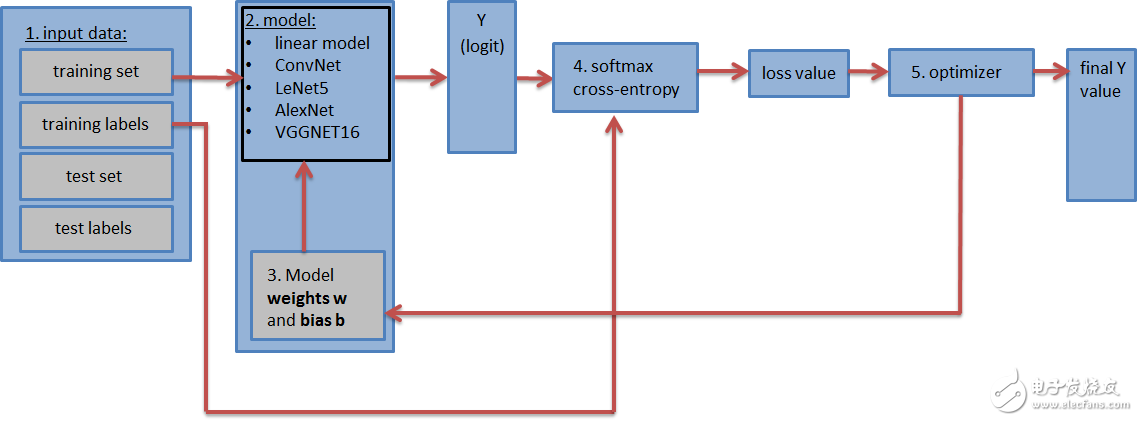
The diagram containing the neural network (shown above) should contain the following steps:
1. Enter data sets: training data sets and labels, test data sets and labels (and validation data sets and labels). The test and validation data sets can be placed in tf.constant(). The training data set is placed in tf.placeholder() so that it can be batched during training (random gradient descent).
2. Neural network** model** and all its layers. This can be a simple fully connected neural network consisting of only one layer or a more complex neural network consisting of 5, 9, and 16 layers.
3. The weight matrix and **deviation vector** are defined and initialized with the appropriate shape. (one weight matrix and deviation vector per layer)
4. Loss value: The model can output a logarithmic vector (estimated training label) and calculate the loss value (softmax with cross entropy function) by comparing the logarithm to the actual label. The loss value indicates how close the estimated training tag is to the actual training tag and is used to update the weight value.
5. Optimizer: It is used to update the calculated loss value to update the weights and deviations in the backpropagation algorithm.
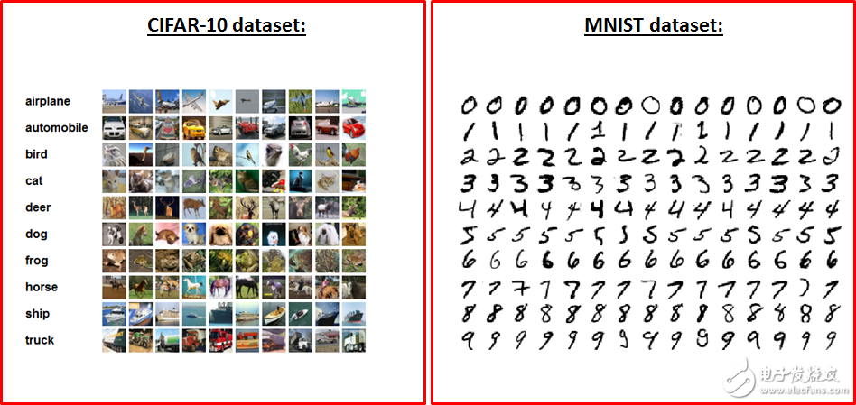
2.2 Data Loading Let's load the data set used to train and test the neural network. To do this, we want to download the MNIST and CIFAR-10 data sets. The MNIST dataset contains 60,000 handwritten digital images, each of which is 28 x 28 x 1 (grayscale). The CIFAR-10 dataset also contains 60,000 images (3 channels) measuring 32 x 32 x 3 and containing 10 different objects (aircraft, car, bird, cat, deer, dog, frog, horse, boat) ,truck). Since there are 10 different objects in both data sets, both data sets contain 10 tags.

First, let's define some methods for loading data and formatting data.
Def randomize(dataset, labels):
permutaTIon = np.random.permutation(labels.shape[0])
Shuffled_dataset = dataset[permutation, :, :]
Shuffled_labels = labels[permutation]
Return shuffled_dataset, shuffled_labels
Def one_hot_encode(np_array):
Return (np.arange(10) == np_array[:,None]).astype(np.float32)
Def reformat_data(dataset, labels, image_width, image_height, image_depth):
Np_dataset_ = np.array([np.array(image_data).reshape(image_width, image_height, image_depth) for image_data in dataset])
Np_labels_ = one_hot_encode(np.array(labels, dtype=np.float32))
Np_dataset, np_labels = randomize(np_dataset_, np_labels_)
Return np_dataset, np_labels
Def flatten_tf_array(array):
Shape = array.get_shape().as_list()
Return tf.reshape(array, [shape[0], shape[1] shape[2] shape[3]])
Def accuracy(predictions, labels):
Return (100.0 * np.sum(np.argmax(predictions, 1) == np.argmax(labels, 1)) / predictions.shape[0])
These methods can be used to encode tags on a single heat code, load data into a random array, and flatten the matrix (since a fully connected network requires a flat matrix as input):
After we have defined these necessary functions, we can load the MNIST and CIFAR-10 data sets like this:
Mnist_folder = './data/mnist/'
Mnist_image_width = 28
Mnist_image_height = 28
Mnist_image_depth = 1
Mnist_num_labels = 10
Mndata = MNIST(mnist_folder)
Mnist_train_dataset_, mnist_train_labels_ = mndata.load_training()
Mnist_test_dataset_, mnist_test_labels_ = mndata.load_testing()
Mnist_train_dataset, mnist_train_labels = reformat_data(mnist_train_dataset_, mnist_train_labels_, mnist_image_size, mnist_image_size, mnist_image_depth)
Mnist_test_dataset, mnist_test_labels = reformat_data(mnist_test_dataset_, mnist_test_labels_, mnist_image_size, mnist_image_size, mnist_image_depth)
Print("There are {} images, each of size {}".format(len(mnist_train_dataset), len(mnist_train_dataset[0])))
Print("Meaning each image has the size of 28281 = {}".format(mnist_image_sizemnist_image_size1))
Print("The training set contains the following {} labels: {}".format(len(np.unique(mnist_train_labels_)), np.unique(mnist_train_labels_)))
Print('Training set shape', mnist_train_dataset.shape, mnist_train_labels.shape)
Print('Test set shape', mnist_test_dataset.shape, mnist_test_labels.shape)
Train_dataset_mnist, train_labels_mnist = mnist_train_dataset, mnist_train_labels
Test_dataset_mnist, test_labels_mnist = mnist_test_dataset, mnist_test_labels
############################################################################ #########################################################
Cifar10_folder = './data/cifar10/'
Train_datasets = ['data_batch_1', 'data_batch_2', 'data_batch_3', 'data_batch_4', 'data_batch_5', ]
Test_dataset = ['test_batch']
C10_image_height = 32
C10_image_width = 32
C10_image_depth = 3
C10_num_labels = 10
With open(cifar10_folder + test_dataset[0], 'rb') as f0:
C10_test_dict = pickle.load(f0, encoding='bytes')
C10_test_dataset, c10_test_labels = c10_test_dict[b'data'], c10_test_dict[b'labels']
Test_dataset_cifar10, test_labels_cifar10 = reformat_data(c10_test_dataset, c10_test_labels, c10_image_size, c10_image_size, c10_image_depth)
C10_train_dataset, c10_train_labels = [], []
For train_dataset in train_datasets:
With open(cifar10_folder + train_dataset, 'rb') as f0:
C10_train_dict = pickle.load(f0, encoding='bytes')
C10_train_dataset_, c10_train_labels_ = c10_train_dict[b'data'], c10_train_dict[b'labels']
C10_train_dataset.append(c10_train_dataset_)
C10_train_labels += c10_train_labels_
C10_train_dataset = np.concatenate(c10_train_dataset, axis=0)
Train_dataset_cifar10, train_labels_cifar10 = reformat_data(c10_train_dataset, c10_train_labels, c10_image_size, c10_image_size, c10_image_depth)
Del c10_train_dataset
Del c10_train_labels
Print("The training set contains the following labels: {}".format(np.unique(c10_train_dict[b'labels'])))
Print('Training set shape', train_dataset_cifar10.shape, train_labels_cifar10.shape)
Print('Test set shape', test_dataset_cifar10.shape, test_labels_cifar10.shape)
You can download the MNIST dataset from the Yann LeCun website. Once downloaded and unzipped, you can use the python-mnist tool to load the data. The CIFAR-10 data set can be downloaded from here.
2.3 Creating a simple layer of neural networks The simplest form of neural networks is a layer of Fully Connected Neural Network (FCNN). Mathematically it consists of a matrix multiplication.
It's best to start with a simple NN in Tensorflow and then study a more complex neural network. When we look at more complex neural networks, only the model (step 2) and weight (step 3) of the graph change, and the other steps remain the same.
We can make a layer of FCNN as follows:
Image_width = mnist_image_width
Image_height = mnist_image_height
Image_depth = mnist_image_depth
Num_labels = mnist_num_labels
#the dataset
Train_dataset = mnist_train_dataset
Train_labels = mnist_train_labels
Test_dataset = mnist_test_dataset
Test_labels = mnist_test_labels
#number of iterations and learning rate
Num_steps = 10001
Display_step = 1000
Learning_rate = 0.5
Graph = tf.Graph()
With graph.as_default():
#1) First we put the input data in a Tensorflow friendly form.
Tf_train_dataset = tf.placeholder(tf.float32, shape=(batch_size, image_width, image_height, image_depth))
Tf_train_labels = tf.placeholder(tf.float32, shape = (batch_size, num_labels))
Tf_test_dataset = tf.constant(test_dataset, tf.float32)
#2) Then, the weight matrices and bias vectors are initialized
#as a default, tf.truncated_normal() is used for the weight matrix and tf.zeros() is used for the bias vector.
Weights = tf.Variable(tf.truncated_normal([image_width image_height image_depth, num_labels]), tf.float32)
Bias = tf.Variable(tf.zeros([num_labels]), tf.float32)
#3) define the model:
#A one layered fccd simply consists of a matrix multiplication
Def model(data, weights, bias):
Return tf.matmul(flatten_tf_array(data), weights) + bias
Logits = model(tf_train_dataset, weights, bias)
#4) calculate the loss, which will be used in the optimization of the weights
Loss = tf.reduce_mean(tf.nn.softmax_cross_entropy_with_logits(logits=logits, labels=tf_train_labels))
#5) Choose an optimizer. Many are available.
Optimizer = tf.train.GradientDescentOptimizer(learning_rate).minimize(loss)
#6) The predicted values ​​for the images in the train dataset and test dataset are assigned to the variables train_prediction and test_prediction.
#It is only necessary if you want to know the accuracy by comparing it with the actual values.
Train_prediction = tf.nn.softmax(logits)
Test_prediction = tf.nn.softmax(model(tf_test_dataset, weights, bias))
With tf.Session(graph=graph) as session:
Tf.global_variables_initializer().run()
Print('Initialized')
For step in range(num_steps):
_, l, predictions = session.run([optimizer, loss, train_prediction])
If (step % display_step == 0):
Train_accuracy = accuracy(predictions, train_labels[:, :])
Test_accuracy = accuracy(test_prediction.eval(), test_labels)
Message = "step {:04d} : loss is {:06.2f}, accuracy on training set {:02.2f} %, accuracy on test set {:02.2f} %".format(step, l, train_accuracy, test_accuracy)
Print(message)
>>> Initialized
>>> step 0000 : loss is 2349.55, accuracy on training set 10.43 %, accuracy on test set 34.12 %
>>> step 0100 : loss is 3612.48, accuracy on training set 89.26 %, accuracy on test set 90.15 %
>>> step 0200 : loss is 2634.40, accuracy on training set 91.10 %, accuracy on test set 91.26 %
>>> step 0300 : loss is 2109.42, accuracy on training set 91.62 %, accuracy on test set 91.56 %
>>> step 0400 : loss is 2093.56, accuracy on training set 91.85 %, accuracy on test set 91.67 %
>>> step 0500 : loss is 2325.58, accuracy on training set 91.83 %, accuracy on test set 91.67 %
>>> step 0600 : loss is 22140.44, accuracy on training set 68.39 %, accuracy on test set 75.06 %
>>> step 0700 : loss is 5920.29, accuracy on training set 83.73 %, accuracy on test set 87.76 %
>>> step 0800 : loss is 9137.66, accuracy on training set 79.72 %, accuracy on test set 83.33 %
>>> step 0900 : loss is 15949.15, accuracy on training set 69.33 %, accuracy on test set 77.05 %
>>> step 1000 : loss is 1758.80, accuracy on training set 92.45 %, accuracy on test set 91.79 %
In the figure, we load the data, define the weight matrix and model, calculate the loss value from the log-log vector, and pass it to the optimizer, which will update the weight of the iteration "num_steps".
In the fully connected NN above, we used a gradient descent optimizer to optimize the weights. However, there are many different optimizers available for Tensorflow. The most commonly used optimizers are GradientDescentOptimizer, AdamOptimizer, and AdaGradOptimizer, so if you are building a CNN, I suggest you try these.
Sebastian Ruder has a nice blog post about the differences between the different optimizers. You can learn more about them in this article.
2.4 Several aspects of Tensorflow
Tensorflow contains many layers, which means that the same operations can be done with different levels of abstraction. Here is a simple example of the operation
Logits = tf.matmul(tf_train_dataset, weights) + biases,
Can also be implemented like this
Logits = tf.nn.xw_plus_b(train_dataset, weights, biases).
This is the most obvious layer in the layers API. It is a highly abstract layer that makes it easy to create neural networks made up of many different layers. For example, or a function is used to create a convolution and a fully connected layer. These functions allow you to specify the number of layers, the size or depth of the filter, the type of the activation function, and so on. Then, the weight matrix and the offset matrix are automatically created, together with the activation function and the dropout regularization laye.
For example, by using the layer API, the following code:
Import Tensorflow as tf
W1 = tf.Variable(tf.truncated_normal([filter_size, filter_size, image_depth, filter_depth], stddev=0.1))
B1 = tf.Variable(tf.zeros([filter_depth]))
Layer1_conv = tf.nn.conv2d(data, w1, [1, 1, 1, 1], padding='SAME')
Layer1_relu = tf.nn.relu(layer1_conv + b1)
Layer1_pool = tf.nn.max_pool(layer1_pool, [1, 2, 2, 1], [1, 2, 2, 1], padding='SAME')
Can be replaced with
From tflearn.layers.conv import conv_2d, max_pool_2d
Layer1_conv = conv_2d(data, filter_depth, filter_size, activation='relu')
Layer1_pool = max_pool_2d(layer1_conv_relu, 2, strides=2)
As you can see, we don't need to define weights, deviations, or activation functions. Especially when you build a neural network with many layers, this keeps the code clear and tidy.
However, if you are new to Tensorflow, it is not appropriate to learn how to build different kinds of neural networks, because tflearn does all the work.
Therefore, we won't use the layer API in this article, but once you fully understand how to build a neural network in Tensorflow, I still recommend using it.
We usually use AVSS, AVS, TXL or cable with generally 18AWG or custom gauge to 16AWG or 14AWG.The connector we recommand is Tyco/AMP/Delphi/Bosch/Deutsch/Yazaki/Sumitomo /Molex replacements or originalTo be applied in automobile or motorcycle HID headlight upgrading system.
We can do any extension cable on GPS Tracking Systems & Driving recorder camera. If you need further question, our profeessional engineers are able to solve for you.
Camera Harness,Camera Wire Harness,Electrical Cable Crimper,Wiring Harness Clips
Dongguan YAC Electric Co,. LTD. , https://www.yacentercn.com